Years ago I noticed that there were a lot of questions on stack overflow about how to track pitch with the FFT. To help out, I wrote a complete, working example of an FFT-based pitch tracker along with this blog post. The code still works, so I’m copying this to my new blog
In this post, I’ll describe a simple, and easy to understand method for tracking pitch, which could be used as a rudimentary guitar tuner. The core of the algorithm is the FFT, or “Fast Fourier transform”, which converts a standard time-domain representation of audio into the frequency domain. The algorithm shown here works, but it converges on the correct pitch slowly and is not super accurate. I’ll suggest a few improvements you could make on the way, but the main focus is understanding the concepts.
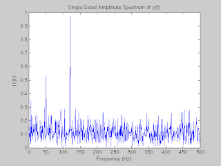
There’s more to getting the algorithm to work than just performing the FFT, though. One example of a potential problem is that every musical instrument creates a multitude of frequencies when one note is played. Each of these is called a “partial” or “harmonic”, and, as shown in the figure, the “fundamental frequency” we are interested in, is not necessarily easy to identify.

Overview
After some basic setup, this pitch detection algorithm I’m presenting is basically a loop on the following steps:
- Read a chunk of audio sample data
- Low-pass the data
- Apply a window to the data
- Transform the data using the FFT
- Find the peak value in the transformed data
- Compute the peak frequency from the index of the peak value in the transformed data
Here is the code that performs these steps:
while( running )
{
    // read some data
    err = Pa_ReadStream( stream, data, FFT_SIZE );

    // low-pass
    for( int j=0; j<FFT_SIZE; ++j ) {
      data[j] = processSecondOrderFilter( data[j], mem1, a, b );
      data[j] = processSecondOrderFilter( data[j], mem2, a, b );
    }
    // window
    applyWindow( window, data, FFT_SIZE );

    // do the fft
    for( int j=0; j<FFT_SIZE; ++j )
      datai[j] = 0;
    applyfft( fft, data, datai, false );

    // find the peak
    float maxVal = -1;
    int maxIndex = -1;
    for( int j=0; j<FFT_SIZE; ++j ) {
      float v = data[j] * data[j] + datai[j] * datai[j] ;
      if( v > maxVal ) {
          maxVal = v;
          maxIndex = j;
      }
    }
    float freq = freqTable[maxIndex];
    //...
}
Let’s go over each of the steps and see how they work.
Audio Data
We always need to start with a sequence of numbers representing the amplitude of audio over time (sometimes called “Linear, PCM audio”). This is what we get from most uncompressed audio formats like AIFF and WAV. Its also what you get from audio APIs like ASIO, CoreAudio and ALSA. In this case, we are using PortAudio, which acts like a portable wrapper around these and other APIs. If you have a compressed format such as MP3 or OGG, you will have to convert it to uncompressed audio first.
Your data might be 16-bit integer, 8-bit integer, 32-bit floating point or any number of other formats. I’ll assume you know how to get your data to floating point representation in the range from -1 to 1. PortAudio takes care of this for us when we specify these input parameters:
inputParameters.device = Pa_GetDefaultInputDevice();
inputParameters.channelCount = 1;
inputParameters.sampleFormat = paFloat32;
inputParameters.suggestedLatency = Pa_GetDeviceInfo( inputParameters.device )->defaultHighInputLatency ;
inputParameters.hostApiSpecificStreamInfo = NULL;
You’ll also need to know how often your audio is sampled. For a tuner, less is more, so we’ll use a sample rate of 8 kHz, which is available on most hardware. This is extremely low for most audio applications (44.1 kHz is considered standard for audio and 48 kHz is standard for video), but for a tuner, 8 kHhz is plenty.
#define SAMPLE_RATE (8000)
Low-Pass Filtering
There’s no hard and fast rule about low-pass filtering (or simply “low-passing”) your audio data. In fact, it’s not even strictly necessary, but doing so can significantly reduce unwanted noise and the higher frequencies that sometimes masquerade as the fundamental frequency. As mentioned in the intro, some instruments have component frequencies called harmonics that are more powerful than the “fundamental” frequency, and for tuning we want to know what the fundamental frequency is. Filtering, therefore, can improve the reliability of the rest of the pitch tracker significantly. Without filtering, some noise might appear to be the dominant pitch, or, more likely, the dominant pitch might appear to be a harmonic of the actual fundamental frequency.
A good choice for the filter is a low-pass filter with a center frequency around the highest pitch you expect to detect. For a guitar tuner, this might be the high E string, which is near 330 Hz, so that’s what we’ll use – in fact, we low-pass it twice. The filter we use is called a 2nd order Butterworth filter. If you are modifying the code for another purpose, you can set the center frequency to something that makes sense for your application.
Windowing
Generally speaking, audio tends to come to us as a long or even continuous stream. Our goal is to get this stream of data into an FFT, which, as we’ll see, works best on small or medium sized chunks of data. To fit this round peg into that square hole, you need to break off chunks of your input, and process the chunks. However, doing so without proper treatment can create noise and distortion.
In rough terms, the problem is that the edges get lopped off very sloppily, creating artifacts at frequencies that aren’t actually present in your signal. These artifacts, called “sidelobes”, cause problems for many applications. Some FFT applications may be designed without special treatment, so in principle you can skip this step, but I strongly recommend you keep reading because it’s easy to deal with this problem.
To reduce the sidelobes, we premultiply each chunk of audio with another signal called a window, or window function. Two simple and popular choices for window functions are the Hamming window, and the Hann window. I put code for both in the tuner, but I used the Hann window.
void buildHanWindow( float *window, int size )
{
  for( int i = 0 to size )
      window[i] = .5 * ( 1 - cos( 2 * M_PI * i / (size-1.0) ) );
}
void applyWindow( float *window, float *data, int size )
{
  for( int i = 0 to size )
      data[i] *= window[i] ;
}
For a tuning app, the windows may overlap, or there may be gaps in between them, depending on your needs and your available processing power. For example, by overlapping and performing more FFTs, and then averaging the results, you may get more accurate results more quickly, at the cost of more CPU time. I strongly recommend doing this in real apps. I did not do this in my app to make the code easier to follow, but it would surely improve the output if overlapping windows were used.
FFT
The FFT, or Fast Fourier Transform, is an algorithm for quickly computing the frequencies that comprise a given signal. By quickly, we mean O( N log N ). This is way faster than the O( N2) of a naive Fourier transform, but still not linear, so you are going to have to be mindful of performance when you use it. In particular, you can’t pass too much data to the FFT at once or it will get very slow. Because the FFT is now the standard way to compute the Fourier transform, many people often use the terms interchangeably, even though this is not strictly correct.
The FFT works on a chunk of samples at a time. You don’t get more or less data out of a Fourier Transform than you put into it, you just get it in another form. That means that if you put ten audio samples in you get ten data-points out. The difference is that these ten data points now represent energy at different frequencies instead of energy at different times, and since our data uses real numbers, and not complex, the FFT will contain some redundancies – specifically, only the first half of the spectrum contains relevant data. That means that for ten samples in, we really only get five relevant data-points out.
Clearly, the more frequency resolution you need, the more time data you need to give it. However, at some point you will run into the problem of not being able to return results quickly enough, either because you are waiting for more input, or because it takes too long to process. Choosing the right size FFT is critical: too big and you consume lots of CPU and delay getting a response, too small and your results lack resolution.
How do we know how big our FFT should be? You can determine the accuracy of your FFT with this simple formula:
binSize = sampleRate/N ;
For example, with a bin size of 8192 (most implementations of the FFT work best with powers of 2), and a sample rate of 44100, you can expect to get results that are accurate to within about 5.38 Hz. Not great for a tuner, but, hey, that’s why we are sampling at 8000 Hz, which gives us an accuracy of better than 1 Hz. Still not perfect, for, say, a 5 string bass, but you can always use a larger N if you need to. Keep in mind that getting enough samples to get more accuracy takes longer than a second, so our display only updates about once a second. That’s yet another reason you might want to overlap your windows.
The output of the FFT is an array of N complex numbers. It is possible to use both the real and imaginary part to get more accurate frequency information, but for now we’ll settle for something simpler and much easier to understand: the magnitude. To find the magnitude of each frequency component, we use the distance formula:
for( i in 0 to N/2 )
  magnitude[i] = sqrt( real[i]*real[i] + cmpx[i]*cmpx[i] );
Now that we know the magnitude of each FFT bin, finding the fundamental frequency is now simply a matter of finding the bin with the maximum magnitude. The frequency will then be the bin number times the bin size, which we computed earlier. (Note that we don’t actually need to compute the square root to find the maximum magnitude, so our actual code skips that step.)
More
You now have the tools to find the fundamental frequency of a single note using the FFT, and a few other tools like windowing and low-pass filtering.
I do a bit more in my code, like identify the nearest semi-tone and find the difference between the that semi-tone and the identified frequency, but for stuff like that I’ll leave the code to speak for itself.


